Machine Learning with Iris Dataset
In this blog-post, we will go through the whole process of creating a Machine Learning model on the famous Iris Flower dataset, which is used by many people all over the world.
Problem Statement
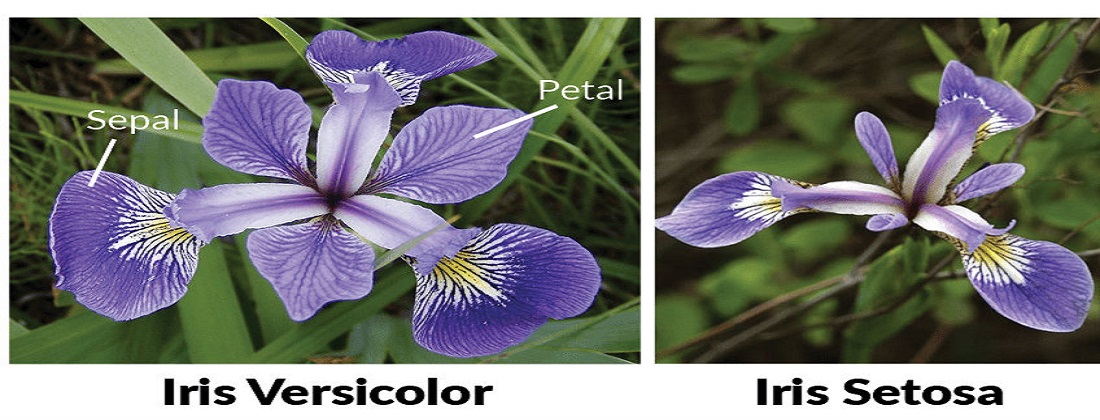
Given Sepal and Petal lengths and width, predict the class of the flower, which could be one of the 3 - Iris setosa, Iris virginica and Iris versicolor.
Dataset Description
The Iris dataset was used in R.A. Fisher’s classic 1936 paper, The Use of Multiple Measurements in Taxonomic Problems, and can also be found on the UCI Machine Learning Repository.
Download link: https://archive.ics.uci.edu/ml/machine-learning-databases/iris/iris.data
The data set consists of 150 rows of 50 samples each of three species of the iris flower with a few columns telling about different features.
#IMAGE#
The columns in this dataset are:
-
Id
-
SepalLengthCm
-
SepalWidthCm
-
PetalLengthCm
-
PetalWidthCm
-
Species (Iris setosa, Iris virginica or Iris versicolor)
Detailed code for the model with more visualizations and code for this tutorial is given at this Page.
Installation
We will be working inside a Jupyter notebook. It will advisable to install anaconda environment on your local machine before proceeding with the task of building any ML model.
To install the Anaconda environment in your local machine you can follow this post: https://medium.com/@margaretmz/anaconda-jupyter-notebook-tensorflow-and-keras-b91f381405f8
Visualizing the Dataset
In this section, let us see how the data distribution looks like.
Here is a brief description of the libraries that we would be using:
-
Numpy: it is used to perform numerical calculations in Python.
-
Pandas: it is used to store data in an organized manner and quickly manipulate it.
-
Matplotlib: it is used to plot data in the form of graphs/charts for visualization.
-
Seaborn: it is a Python data visualization library based on Matplotlib
import numpy as np
import pandas as pd
import matplotlib.pyplot as plt
import seaborn as sns
#import the dataset
iris = pd.read_csv("Iris.csv")
#Let's have a look at the dataset
iris.head()

We can see that there are three species of Iris flower present in the dataset with 50 samples each. Remember that Machine Learning is not a magic branch of Computer Science. The predictions are always data driven. Without data, there is no value to data science or Machine Learning. More the data, better the accuracy.
Understanding the data distribution of a given database before applying any Machine Learning technique is the most important step of the analysis.
Most of the algorithms of Machine Learning consider, either explicit or implicit, a certain number of assumptions about the input data and only work accurately if these assumptions hold. If those assumptions don't hold, the result may be meaningless.
For example, for simple linear regression, the assumptions are,
-
Additivity and linearity of effects
-
Constant error variance
-
The normality of errors and zero correlation between errors.
|
sns.set_style('whitegrid'); |
#IMAGE#
The iris-setosa is linearly separable from iris-versicolor and iris-virginica. We have to devise some method to separate all these labels with an appropriate decision boundary so that prediction can be accurate.
Let’s see some pair plots and observe if we can get some insights.
|
plt.close();
|

Observations:
-
Using sepal_length and sepal_width features, we can distinguish Setosa flowers from others.
-
Separating Versicolor from Viginica is much harder as they have considerable overlap.
Let’s look at some histograms to check the probability distribution of the flower samples based on the features given.
In probability theory and statistics, a probability distribution is a mathematical function that provides the probabilities of occurrence of different possible outcomes in an experiment. In more technical terms, the probability distribution is a description of a random phenomenon in terms of the probabilities of events. For instance, if the random variable X is used to denote the outcome of a coin toss ("the experiment"), then the probability distribution of X would take the value 0.5 for X = heads, and 0.5 for X = tails (assuming the coin is fair). Examples of random phenomena can include the results of an experiment or survey.
|
sns.FacetGrid(iris, hue= 'Species', size= 5)\
sns.FacetGrid(iris, hue= 'Species', size= 5)\ .map(sns.distplot, "SepalLengthCm")\ .add_legend() plt.show()
|


We can see that the distribution is very much overlapped when Sepal length was taken into account in comparison to Petal length. This clearly indicates that Petal features are much more appropriate in making the predictive analysis.
Let’s see the statistical values like mean, standard deviation and median for Petal Length.
print("Mean for setosa's petal length is {}".format(np.mean(iris_setosa['PetalLengthCm'])))
print("Mean for versicolor's petal length is {}".format(np.mean(iris_versicolor['PetalLengthCm'])))
print("Mean for virginica's petal length is {}".format(np.mean(iris_virginica['PetalLengthCm'])))
Mean for setosa's petal length is 1.464
Mean for versicolor's petal length is 4.26
Mean for virginica's petal length is 5.5520000000000005
print("Std-dev for setosa's petal length is {}".format(np.std(iris_setosa['PetalLengthCm'])))
print("Std-dev for versicolor's petal length is {}".format(np.std(iris_versicolor['PetalLengthCm'])))
print("Std-dev for virginica's petal length is {}".format(np.std(iris_virginica['PetalLengthCm'])))
Std-dev for setosa's petal length is 0.17176728442867112
Std-dev for versicolor's petal length is 0.4651881339845203
Std-dev for virginica's petal length is 0.546347874526844
print("Median for setosa's petal length is {}".format(np.median(iris_setosa['PetalLengthCm'])))
print("Median for versicolor's petal length is {}".format(np.median(iris_versicolor['PetalLengthCm'])))
print("Median for virginica's petal length is {}".format(np.median(iris_virginica['PetalLengthCm'])))
Median for setosa's petal length is 1.5
Median for versicolor's petal length is 4.35
Median for virginica's petal length is 5.55
Building the Model:
We will be using:
-
Logistic Regression
-
Linear SVM
-
Feedforward Neural Network
To train our model.
Let’s import the necessary metrics and libraries.
Linear Regression
from sklearn.model_selection import train_test_split
from sklearn.metrics import confusion_matrix, accuracy_score
from sklearn.linear_model import LogisticRegression
X= iris.iloc[:, 0:4]
y= iris.iloc[:, 4]
X_train,X_test,y_train,y_test= train_test_split(X, y, test_size= 0.15, random_state= 1)
model_lr = LogisticRegression()
model_lr.fit(X_train, y_train)
pred_lr = model_lr.predict(X_test)
print("Accuracy Using Logistic Regression is {}".format(accuracy_score(y_test, pred_lr)))
Accuracy Using Logistic Regression is 0.782608695652174
Linear SVM
from sklearn.svm import SVC
model_s = SVC()
model_s.fit(X_train, y_train)
pred_s = model_s.predict(X_test)
print("Accuracy Using SVM is {}".format(accuracy_score(y_test, pred_s)))
Accuracy Using SVM is 0.9565217391304348
We can see that Linear SVM is doing great work in making predictions even when the dataset was less. We can use only Petal features in our dataset to predict the class label.
Let’s see the result of a linear SVM model on a dataset containing only Petal Length and Petal Width as features.
Xp = iris.iloc[:, 2:4]
yp = iris.iloc[:, 4]
X_train,X_test,y_train,y_test= train_test_split(Xp, yp, test_size= 0.15, random_state= 1)
model_s2 = SVC()
model_s2.fit(X_train, y_train)
pred_s2 = model_s2.predict(X_test)
print("Accuracy Using SVM is {}".format(accuracy_score(y_test, pred_s2)))
Accuracy Using SVM is 0.9565217391304348
As we can see that the accuracy is similar to the accuracy by previous linear SVM model. This tells that even the lesser number of most important features can accurately learn the variations of a dataset and can make accurate predictions.
Neural Network
import torch
from torch import nn
from sklearn.preprocessing import normalize
from torch import optim
import torch.nn.functional as F
for i in range(len(y)):
if y[i] == 'Iris-setosa':
y[i] = 0
elif y[i] == 'Iris-versicolor':
y[i] = 1
else:
y[i] = 2
X = normalize(X)
y = np.array(y)
y = y.astype(int)
X_train,X_test,y_train,y_test= train_test_split(X, y, test_size= 0.10, random_state= 1)
model=nn.Sequential(nn.Linear(4,27),nn.ReLU(),nn.Linear(27,9),nn.ReLU(),nn.Linear(9,3),nn.LogSoftmax(dim= 1))
criterion = nn.NLLLoss()
optimizer = optim.SGD(model.parameters(), lr=0.003)
def train(model, criterion, optimizer, inputs, labels):
optimizer.zero_grad()
output = model(inputs)
loss = criterion(output, labels)
loss.backward()
optimizer.step()
return loss.item()
def predict(model, inputs):
output = model(inputs)
return output.data.numpy().argmax(axis= 1)
X_train = torch.from_numpy(X_train).float()
X_test = torch.from_numpy(X_test).float()
y_train = torch.from_numpy(y_train).long()
epochs= 100
batch_size= 15
n_batches = 9
costs = []
test_accuracies = []
for e in range(epochs):
running_loss = 0
for j in range(n_batches):
Xbatch = X_train[j*batch_size:(j+1)*batch_size]
Ybatch = y_train[j*batch_size:(j+1)*batch_size]
running_loss += train(model, criterion, optimizer, Xbatch, Ybatch)
Ypred = predict(model, X_test)
acc = np.mean(y_test == Ypred)
print("Epoch:%d,cost:%f,accuracy:%.2f"%(e,running_loss/n_batches,acc))
costs.append(running_loss/n_batches)
test_accuracies.append(acc)
ypred = predict(model, X_test)
from sklearn.metrics import confusion_matrix, accuracy_score
print("Accuracy Score is {}".format(accuracy_score(y_test, ypred)))
Accuracy Score is 0.3333333333333333
We trained a feed-forward neural network too on the dataset using PyTorch but the accuracy was just 33% due to the lesser quantity of the quality dataset.
We have shown you how to approach a dataset by exploring it using Exploratory Data Analysis and then building the model to predict the results.
Keep Learning!!!
Detailed code for the model with more visualizations and code for this tutorial is given at this Page.


